Open-Loop Storage Controllers Demonstrations#
from pathlib import Path
from matplotlib import pyplot as plt
from h2integrate.core.h2integrate_model import H2IntegrateModel
from h2integrate import EXAMPLE_DIR
Hydrogen Dispatch#
The following example is an expanded form of examples/14_wind_hydrogen_dispatch.
Here, we’re highlighting the dispatch controller setup from
examples/14_wind_hydrogen_dispatch/inputs/tech_config.yaml. Please note some sections are removed simply to highlight the controller sections
52  h2_storage:
53    performance_model:
54      model: StoragePerformanceModel
55    control_strategy:
56      model: DemandOpenLoopStorageController
57    model_inputs:
58      shared_parameters:
59        commodity: hydrogen
60        commodity_rate_units: kg/h
61        max_charge_rate: 12446.00729773  # kg/time step
62        max_capacity: 2987042.0  # kg
63        max_soc_fraction: 1.0  # fraction (0-1)
64        min_soc_fraction: 0.1  # fraction (0-1)
65        init_soc_fraction: 0.25  # fraction (0-1)
66        max_discharge_rate: 12446.00729773  # kg/time step
67        charge_efficiency: 1.0  # fraction (0-1)
68        discharge_efficiency: 1.0  # fraction (0-1)
69        demand_profile: 5000  # constant demand of 5000 kg per hour (see commodity_rate_units)
We also include a demand technology to calculate how much demand is met, how much commodity is unused to meet the demand, and how much demand is remaining:
79  h2_load_demand:
80    performance_model:
81      model: GenericDemandComponent
82    model_inputs:
83      performance_parameters:
84        commodity: hydrogen
85        commodity_rate_units: kg/h
86        demand_profile: 5000  # 5000 kg/h
Using the primary configuration, we can create, run, and postprocess an H2Integrate model.
# Create an H2Integrate model
model = H2IntegrateModel(EXAMPLE_DIR/"14_wind_hydrogen_dispatch"/"inputs"/"h2i_wind_to_h2_storage.yaml")

# Run the model
model.run()
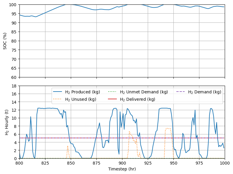
Now, we can visualize the demand profiles over time.
fig, (ax1, ax2) = plt.subplots(2, 1, sharex=True, figsize=(8, 6), layout="tight")

start_hour = 800
end_hour = 1000
xvals = list(range(start_hour, end_hour))

ax1.plot(
    xvals,
    model.prob.get_val("h2_storage.SOC", units="percent")[start_hour:end_hour],
    label="SOC",
)
ax2.plot(
    xvals,
    model.prob.get_val("h2_storage.hydrogen_in", units="t/h")[start_hour:end_hour],
    linestyle="-",
    label="H$_2$ Produced (kg)",
)
ax2.plot(
    xvals,
    model.prob.get_val("h2_load_demand.unused_hydrogen_out", units="t/h")[start_hour:end_hour],
    linestyle=":",
    label="H$_2$ Unused (kg)",
)
ax2.plot(
    xvals,
    model.prob.get_val("h2_load_demand.unmet_hydrogen_demand_out", units="t/h")[start_hour:end_hour],
    linestyle=":",
    label="H$_2$ Unmet Demand (kg)",
)
ax2.plot(
    xvals,
    model.prob.get_val("h2_load_demand.hydrogen_out", units="t/h")[start_hour:end_hour],
    linestyle="-",
    label="H$_2$ Delivered (kg)",
)
ax2.plot(
    xvals,
    model.prob.get_val("h2_load_demand.hydrogen_demand", units="t/h")[start_hour:end_hour],
    linestyle="--",
    label="H$_2$ Demand (kg)",
)

ax1.set_ylabel("SOC (%)")
ax1.grid()
ax1.set_axisbelow(True)
ax1.set_xlim(start_hour, end_hour)
ax1.set_ylim(60, 100)

ax2.set_ylabel("H$_2$ Hourly (t)")
ax2.set_xlabel("Timestep (hr)")
ax2.grid()
ax2.set_axisbelow(True)
ax2.set_ylim(0, 18)
ax2.set_yticks(range(0, 19, 2))

plt.legend(ncol=3)
fig.show()