Demand Demonstration#
Different usage of demand components are shown in the following examples:
13_dispatch_for_electrolyzer: showcases how to set an overall demand for the system and a separate demand for the battery system.23_solar_wind_ng_demand: compares usage of theGenericDemandComponentandFlexibleDemandComponent.24_solar_battery_grid: highlights how to sell the electricity in excess of the demand to the grid.
This demonstration will focus on the 13_dispatch_for_electrolyzer example
Electrolyzer load demand#
The following example is an expanded form of examples/13_dispatch_for_electrolyzer.
The technology interconnections:
16technology_interconnections:
17  # combine the generation and input it to the battery
18  - [distributed_wind_plant, gen_combiner, electricity, cable]
19  - [distributed_pv, gen_combiner, electricity, cable]
20  - [gen_combiner, battery, electricity, cable]
21  # combine the battery output with the wind and solar generation
22  - [battery, elec_combiner, electricity, cable]
23  - [gen_combiner, elec_combiner, electricity, cable]
24  # subtract the electricity generated from the electricity demand
25  - [elec_combiner, elec_load_demand, electricity, cable]
26  # connect the electricity supplied to the demand to the electrolyzer
27  - [elec_load_demand, electrolyzer, electricity, cable]
Which we can visualize using an XDSM diagram:

The electrolyzer system is comprised of 6 stacks, each rated at 10 MW, resulting in a total capacity of 60 MW. The minimum operating point of the electrolyzer (turndown_ratio) is 10% of the rated capacity, meaning that the electrolyzer is turned off if there is less than 6 MW of input electricity.
120  electrolyzer:
121    performance_model:
122      model: ECOElectrolyzerPerformanceModel
123    cost_model:
124    model_inputs:
125      performance_parameters:
126        n_clusters: 6  # number of 10 MW clusters
127        cluster_rating_MW: 10  # 10 MW clusters
128        turndown_ratio: 0.1  # turndown_ratio = minimum_cluster_power/cluster_rating_MW
We want to dispatch the battery to keep the electrolyzer on. We set the demand profile for the battery as the minimum power required to keep the electrolyzer on, 6 MW.
Note
Note: the demand profile for the battery is only used by the battery controller and is not used in the battery performance model for any calculations.
79  battery:
80    performance_model:
81      model: StoragePerformanceModel
82    cost_model:
83      model: GenericStorageCostModel
84    control_strategy:
85      model: DemandOpenLoopStorageController
86    model_inputs:
87      shared_parameters:
88        commodity: electricity
89        commodity_rate_units: MW
90        commodity_amount_units: MW*h
91        demand_profile: 6.0  # equal to electrolyzer turndown ratio (6 MW)
We don’t want to send more electricity to the electrolyzer than the electrolyzer can use. We use the demand component to saturate the electricity generation to the electrolyzer’s rated capacity (equal to 60 MW).
112  elec_load_demand:  # load demand component for electrolyzer
113    performance_model:
114      model: GenericDemandComponent
115    model_inputs:
116      performance_parameters:
117        commodity: electricity
118        commodity_rate_units: MW
119        demand_profile: 60  # Equal to electrolyzer capacity
We initialize and setup the H2I model
from pathlib import Path
from matplotlib import pyplot as plt
from h2integrate.core.h2integrate_model import H2IntegrateModel
from h2integrate import EXAMPLE_DIR
from h2integrate.core.inputs.validation import load_tech_yaml, load_plant_yaml, load_driver_yaml

ex_dir = EXAMPLE_DIR / "13_dispatch_for_electrolyzer"
tech_config = load_tech_yaml(ex_dir / "tech_config.yaml")
plant_config = load_plant_yaml(ex_dir / "plant_config.yaml")
driver_config = load_driver_yaml(ex_dir / "driver_config.yaml")

# modify all the output folders to be full filepaths
driver_config["general"]["folder_output"] = str(Path(ex_dir / "outputs").absolute())
tech_config["technologies"]["distributed_wind_plant"]["model_inputs"]["performance_parameters"][
    "cache_dir"
] = ex_dir / "cache"

input_config = {
    "plant_config": plant_config,
    "technology_config": tech_config,
    "driver_config": driver_config,
}


# Create an H2Integrate model
h2i = H2IntegrateModel(input_config)

# Setup the model
h2i.setup()
If we wanted to change the demand profiles for the battery (battery) or the demand component (elec_load_demand) to be different than the demand profiles specified in the technology config, we could do that using set_val:
electrolyzer_capacity_MW = 60

## Set the battery demand equal to the minimum electricity needed to keep the electrolyzer on
# h2i.prob.set_val("battery.electricity_demand", 0.1 * electrolyzer_capacity_MW, units="MW")

## Set the demand of the demand component equal to the rated electrical capacity of the electrolyzer
# h2i.prob.set_val("elec_load_demand.electricity_demand", electrolyzer_capacity_MW, units="MW")
We then run the model:
# Run the model
h2i.run()
h2i.prob.get_val("finance_subgroup_hydrogen.LCOH", units="USD/kg")[0]
/home/docs/checkouts/readthedocs.org/user_builds/h2integrate/envs/latest/lib/python3.11/site-packages/floris/core/flow_field.py:156: UserWarning: 'where' used without 'out', expect unitialized memory in output. If this is intentional, use out=None.
  * np.power(
np.float64(16.030903274742947)
Plotting outputs#
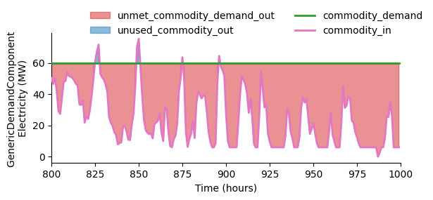
First, we get the main inputs and outputs of the GenericDemandComponent technology:
generation_with_battery = h2i.prob.get_val("elec_load_demand.electricity_in", units="MW")
full_demand = h2i.prob.get_val("elec_load_demand.electricity_demand", units="MW")
unmet_demand = h2i.prob.get_val("elec_load_demand.unmet_electricity_demand_out", units="MW")
excess_electricity = h2i.prob.get_val("elec_load_demand.unused_electricity_out", units="MW")
Plot the inputs to the GenericDemandComponent and outputs calculated in the GenericDemandComponent:
import matplotlib.pyplot as plt
fig, ax = plt.subplots(1, 1, figsize=[6.4, 2.4])

start_hour = 800
end_hour = 1000

x = list(range(start_hour, end_hour))
where_unmet_demand = [True if d>0 else False for d in unmet_demand[start_hour:end_hour]]
where_excess_commodity = [True if d>0 else False for d in excess_electricity[start_hour:end_hour]]

ax.fill_between(x, full_demand[start_hour:end_hour], generation_with_battery[start_hour:end_hour], where=where_unmet_demand, color="tab:red", alpha=0.5, zorder=0, label="unmet_commodity_demand_out")
ax.fill_between(x, full_demand[start_hour:end_hour], generation_with_battery[start_hour:end_hour], where=where_excess_commodity, color="tab:blue", alpha=0.5, zorder=1, label="unused_commodity_out")
ax.plot(x, full_demand[start_hour:end_hour], color="tab:green", lw=2.0, ls='solid', zorder=4, label="commodity_demand")
ax.plot(x, generation_with_battery[start_hour:end_hour], color="tab:pink", lw=2.0, ls='solid', zorder=3, label="commodity_in")

ax.set_xlim([start_hour,end_hour])
ax.spines[['right', 'top']].set_visible(False)
ax.legend(bbox_to_anchor=(0.10, 0.95), loc="lower left", borderaxespad=0.0, framealpha=0.0,  ncols=2)
ax.set_ylabel("GenericDemandComponent \nElectricity (MW)")
ax.set_xlabel("Time (hours)")
Text(0.5, 0, 'Time (hours)')
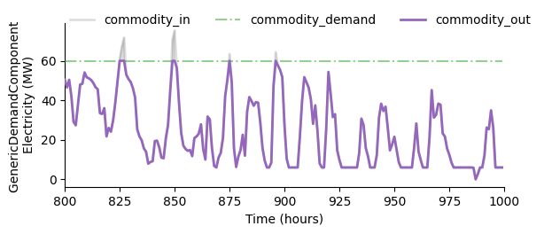
Plot the main inputs and outputs of the GenericDemandComponent:
fig, ax = plt.subplots(1, 1, figsize=[6.4, 2.4])
ax.fill_between(x, full_demand[start_hour:end_hour], generation_with_battery[start_hour:end_hour], where=where_excess_commodity, color="tab:grey", alpha=0.25, zorder=1, label="_unused_commodity_out")
ax.plot(x, generation_with_battery[start_hour:end_hour], color="tab:grey", lw=2.0, ls='solid', zorder=2, label="commodity_in", alpha=0.25)

ax.plot(x, full_demand[start_hour:end_hour], color="tab:green", alpha=0.5, lw=1.5, ls='-.', zorder=3, label="commodity_demand")

ax.plot(x, h2i.prob.get_val("elec_load_demand.electricity_out", units="MW")[start_hour:end_hour], color="tab:purple", lw=2.0, ls='solid', zorder=4, label="commodity_out")
ax.spines[['right', 'top']].set_visible(False)
ax.set_xlim([start_hour, end_hour])
ax.set_ylabel("GenericDemandComponent \nElectricity (MW)")
ax.set_xlabel("Time (hours)")
ax.legend(bbox_to_anchor=(0.0, 0.95), loc="lower left", ncols=3, borderaxespad=0.0, framealpha=0.0)
<matplotlib.legend.Legend at 0x77374ba90b10>
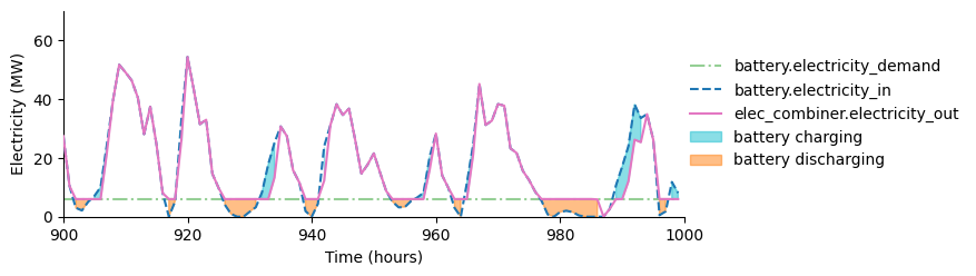
Plot the battery performance:
fig, ax = plt.subplots(1, 1, figsize=[7.2, 2.4])

start_hour = 900
end_hour = 1000
x = list(range(start_hour, end_hour))

generation = h2i.prob.get_val("battery.electricity_in", units="MW")
battery_demand = h2i.prob.get_val("battery.electricity_demand", units="MW")
battery_charge_discharge = h2i.prob.get_val("battery.electricity_out", units="MW")

where_charge =  [True if d<0 else False for d in battery_charge_discharge[start_hour:end_hour]]
where_discharge =  [True if d>0 else False for d in battery_charge_discharge[start_hour:end_hour]]

ax.plot(x, battery_demand[start_hour:end_hour], color="tab:green", alpha=0.5, lw=1.5, ls='-.', zorder=2, label="battery.electricity_demand")
ax.plot(x, generation[start_hour:end_hour], color="tab:blue", alpha=1.0, lw=1.5, ls='--', zorder=3, label="battery.electricity_in")
ax.plot(x, generation_with_battery[start_hour:end_hour], color="tab:pink", alpha=1.0, lw=1.5, ls='-', zorder=3, label="elec_combiner.electricity_out")
ax.fill_between(x, generation[start_hour:end_hour], generation_with_battery[start_hour:end_hour], where=where_charge, color="tab:cyan", alpha=0.5, zorder=0, label="battery charging")
ax.fill_between(x, generation[start_hour:end_hour], generation_with_battery[start_hour:end_hour], where=where_discharge, color="tab:orange", alpha=0.5, zorder=0, label="battery discharging")


ax.spines[['right', 'top']].set_visible(False)
ax.set_xlim([start_hour, end_hour])
ax.set_ylim([0, 70])
ax.legend(bbox_to_anchor=(1.0, 0.5), loc="center left", borderaxespad=0, framealpha=0.0)
ax.set_ylabel("Electricity (MW)")
ax.set_xlabel("Time (hours)")
Text(0.5, 0, 'Time (hours)')
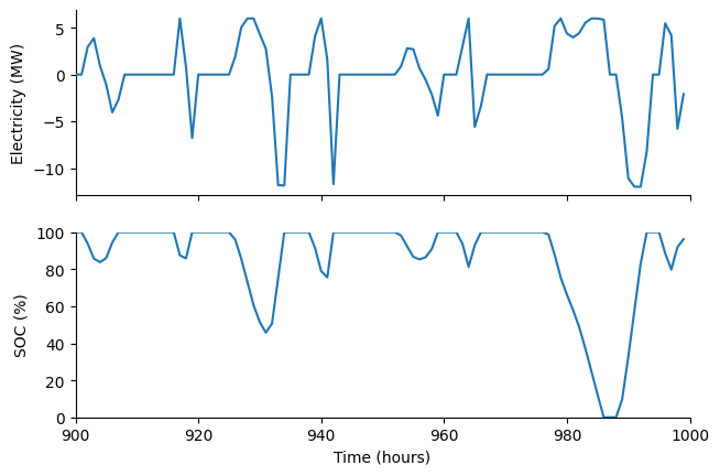
Plot the battery SOC and charge/discharge profile
fig, (ax1, ax2) = plt.subplots(2, 1, sharex=True, figsize=[7.2, 4.8])

battery_SOC = h2i.prob.get_val("battery.SOC", units="percent")

ax1.plot(x, battery_charge_discharge[start_hour:end_hour], color="tab:blue", alpha=1.0, lw=1.5, ls='-', zorder=3, label="battery.electricity_out")
ax1.spines[['right', 'top']].set_visible(False)
ax1.set_xlim([start_hour, end_hour])
ax.legend(bbox_to_anchor=(1.0, 0.5), loc="center left", borderaxespad=0, framealpha=0.0)
ax1.set_ylabel("Electricity (MW)")


# Plot the SOC
ax2.plot(x, battery_SOC[start_hour:end_hour], color="tab:blue", lw=1.5)

ax2.set_ylabel("SOC (%)")
ax2.set_ylim([0, 100])
ax2.spines[['right', 'top']].set_visible(False)
ax2.set_xlabel("Time (hours)")
Text(0.5, 0, 'Time (hours)')
Changing the battery demand#
Lets see what the LCOH is when the battery is used to keep the electrolyzer on:
h2i.prob.get_val("finance_subgroup_hydrogen.LCOH", units="USD/kg")[0]
np.float64(16.030903274742947)
If we re-run H2I and set the battery demand equal to the electrolyzer capacity instead, we can see that the LCOH increases:
# Set the battery demand equal to the rated electrical capacity of the electrolyzer
h2i.prob.set_val("battery.electricity_demand",electrolyzer_capacity_MW, units="MW")

# Set the demand of the demand component equal to the rated electrical capacity of the electrolyzer
h2i.prob.set_val("elec_load_demand.electricity_demand", electrolyzer_capacity_MW, units="MW")

# Re-run H2I
h2i.run()

# Get the LCOH
h2i.prob.get_val("finance_subgroup_hydrogen.LCOH", units="USD/kg")[0]
np.float64(17.217682367493282)