How to set up an analysis#
H2Integrate is designed so that you can run a basic analysis or design problem without extensive Python experience. The key inputs for the analysis are the configuration files, which are in YAML format. This doc page will walk you through the steps to set up a basic analysis, focusing on the different types of configuration files and how use them.
Top-level config file#
The top-level config file is the main entry point for H2Integrate. Its main purpose is to define the analysis type and the configuration files for the different components of the analysis. Here is an example of a top-level config file:
1name: H2Integrate Config
2system_summary: This reference hybrid plant...
3driver_config: driver_config.yaml
4technology_config: tech_config.yaml
5plant_config: plant_config.yaml
The top-level config file contains the following keys:
name: (optional) A name for the analysis. This is used to identify the analysis in the output files.system_summary: (optional) A summary of the analysis. This helpful for quickly describing the analysis for documentation purposes.driver_config: The path to the driver config file. This file defines the analysis type and the optimization settings.technology_config: The path to the technology config file. This file defines the technologies included in the analysis, their modeling parameters, and the performance, cost, and financial models used for each technology.plant_config: The path to the plant config file. This file defines the system configuration and how the technologies are connected together.
The goal of the organization of the top-level config file is that it is easy to swap out different configurations for the analysis without having to change the code.
For example, if you had different optimization problems, you could have different driver config files for each optimization problem and just change the driver_config key in the top-level config file to point to the new file.
This allows you to quickly test different configurations and see how they affect the results.
Note
The filepaths for the plant_config, tech_config, and driver_config files specified in the top-level config file can be specified as either:
Filepaths relative to the top-level config file; this is done in most examples
Filepaths relative to the current working directory; this is also done in most examples, which are intended to be run from the folder they’re in.
Filepaths relative to the H2Integrate root directory; this works best for unique filenames.
Absolute filepaths.
More information about file handling in H2I can be found here
Driver config file#
The driver config file defines the analysis type and the optimization settings. If you are running a basic analysis and not an optimization, the driver config file is quite straightforward and might look like this:
 1name: driver_config
 2description: This analysis runs a wind plant hooked up to an electrolyzer and simple tank
 3general:
 4  folder_output: wind_electrolyzer
 5recorder:
 6  # required inputs
 7  flag: true  # record outputs
 8  file: cases.sql  # this file will be written to the folder `wind_electrolyzer`
 9
10  # optional but recommended inputs
11  overwrite_recorder: true  # If True, do not create a unique recorder file for subsequent runs. Defaults to False.
12  recorder_attachment: model  #"driver" or "model", defaults to "model". Use "driver" if running a parallel simulation.
13  includes: ['*'] #include everything
14  excludes: ['*wind_resource*'] #exclude wind resource data
15
16  # below are optional and defaulted to the OpenMDAO default
17  # record_inputs: True  # defaults to True
18  # record_outputs: True  # defaults to True
19  # record_residuals: True  # defaults to True
20  # options_excludes: # this is only used if recorder_attachment is "model"
If you are running an optimization, the driver config file will contain additional keys to define the optimization settings, including design variables, constraints, and objective functions. Further details of more complex instances of the driver config file can be found in more advanced examples as they are developed.
Technology config file#
The technology config file defines the technologies included in the analysis, their modeling parameters, and the performance, cost, and financial models used for each technology.
The yaml file is organized into sections for each technology included in the analysis under the technologies heading.
Here is an example of a technology config that is defining an energy system with wind and electrolyzer technologies:
 1name: technology_config
 2description: This plant has wind feeding into an electrolyzer without optimization
 3technologies:
 4  wind:
 5    performance_model:
 6      model: PYSAMWindPlantPerformanceModel
 7    cost_model:
 8      model: ATBWindPlantCostModel
 9    model_inputs:
10      performance_parameters:
11        num_turbines: 100
12        turbine_rating_kw: 8300
13        rotor_diameter: 196.
14        hub_height: 130.
15        create_model_from: default
16        config_name: WindPowerSingleOwner
17        pysam_options: !include "pysam_options_8.3MW.yaml"
18        run_recalculate_power_curve: false
19        layout:
20          layout_mode: basicgrid
21          layout_options:
22            row_D_spacing: 10.0
23            turbine_D_spacing: 10.0
24            rotation_angle_deg: 0.0
25            row_phase_offset: 0.0
26            layout_shape: square
27      cost_parameters:
28        capex_per_kW: 1500.0
29        opex_per_kW_per_year: 45
30        cost_year: 2019
31  electrolyzer:
32    performance_model:
33      model: ECOElectrolyzerPerformanceModel
34    cost_model:
35      model: SingliticoCostModel
36    model_inputs:
37      shared_parameters:
38        location: onshore
39        electrolyzer_capex: 1295  # $/kW overnight installed capital costs for a 1 MW system in 2022
40      performance_parameters:
41        size_mode: normal
42        n_clusters: 13  # should be 12.5 to get 500 MW
43        cluster_rating_MW: 40
44        eol_eff_percent_loss: 13  # eol defined as x% change in efficiency from bol
45        uptime_hours_until_eol: 80000.  # number of 'on' hours until electrolyzer reaches eol
46        include_degradation_penalty: true  # include degradation
47        turndown_ratio: 0.1  # turndown_ratio = minimum_cluster_power/cluster_rating_MW
48      financial_parameters:
49        capital_items:
50          depr_period: 7  # based on PEM Electrolysis H2A Production Case Study Documentation estimate of 7 years.
51          replacement_cost_percent: 0.15  # percent of capex - H2A default case
Here, we have defined a wind plant using the pysam_wind_plant_performance and atb_wind_cost models, and an electrolyzer using the eco_pem_electrolyzer_performance and singlitico_electrolyzer_cost models.
The performance_model and cost_model keys define the models used for the performance and cost calculations, respectively.
The model_inputs key contains the inputs for the models, which are organized into sections for shared parameters, performance parameters, cost parameters, and financial parameters.
The shared_parameters section contains parameters that are common to all models, such as the rating and location of the technology.
These values are defined once in the shared_parameters section and are used by all models that reference them.
The performance_parameters section contains parameters that are specific to the performance model, such as the sizing and efficiency of the technology.
The cost_parameters section contains parameters that are specific to the cost model, such as the capital costs and replacement costs.
The financial_parameters section contains parameters that are specific to the financial model, such as the replacement costs and financing terms.
Note
There are no default values for the parameters in the technology config file. You must define all the parameters for the models you are using in the analysis.
Based on which models you choose to use, the inputs will vary.
Each model has its own set of inputs, which are defined in the source code for the model.
Because there are no default values for the parameters, we suggest you look at an existing example that uses the model you are interested in to see what inputs are required or look at the source code for the model.
The different models are defined in the supported_models.py file in the h2integrate package.
Plant config file#
The plant config file defines the system configuration, any parameters that might be shared across technologies, and how the technologies are connected together.
Here is an example plant config file:
 1name: plant_config
 2description: This plant is located in CO, USA...
 3sites:
 4  site:
 5    latitude: 35.2018863
 6    longitude: -101.945027
 7    resources:
 8      wind_resource:
 9        resource_model: WTKNLRDeveloperAPIWindResource
10        resource_parameters:
11          resource_year: 2012
12plant:
13  plant_life: 30
14technology_interconnections: [[wind, electrolyzer, electricity, cable]]
15resource_to_tech_connections: [[site.wind_resource, wind, wind_resource_data]]
16finance_parameters:
17  finance_groups:
18    custom_model:
19      finance_model: simple_lco_finance
20      finance_model_class_name: SimpleLCOFinance
21      finance_model_location: user_finance_model/simple_lco.py
22      model_inputs:
23        discount_rate: 0.09
24    profast_model:
25      finance_model: ProFastLCO
26      model_inputs:
27        params:
28          analysis_start_year: 2032
29          installation_time: 36  # months
30          inflation_rate: 0.0  # 0 for nominal analysis
31          discount_rate: 0.09  # nominal return based on 2024 ATB baseline workbook for land-based wind
32          debt_equity_ratio: 2.62  # 2024 ATB uses 72.4% debt for land-based wind
33          property_tax_and_insurance: 0.03  # percent of CAPEX estimated based on https://www.nrel.gov/docs/fy25osti/91775.pdf https://www.house.mn.gov/hrd/issinfo/clsrates.aspx
34          total_income_tax_rate: 0.257  # 0.257 tax rate in 2024 atb baseline workbook, value here is based on federal (21%) and state in MN (9.8)
35          capital_gains_tax_rate: 0.15  # H2FAST default
36          sales_tax_rate: 0.07375  # total state and local sales tax in St. Louis County https://taxmaps.state.mn.us/salestax/
37          debt_interest_rate: 0.07  # based on 2024 ATB nominal interest rate for land-based wind
38          debt_type: Revolving debt  # can be "Revolving debt" or "One time loan". Revolving debt is H2FAST default and leads to much lower LCOH
39          loan_period_if_used: 0  # H2FAST default, not used for revolving debt
40          cash_onhand_months: 1  # H2FAST default
41          admin_expense: 0.00  # percent of sales H2FAST default
42        capital_items:
43          depr_type: MACRS   # can be "MACRS" or "Straight line"
44          depr_period: 5  # 5  years - for clean energy facilities as specified by the IRS MACRS schedule https://www.irs.gov/publications/p946#en_US_2020_publink1000107507
45          refurb: [0.]
46  finance_subgroups:
47    electricity_profast:
48      commodity: electricity
49      # commodity_stream: "wind"
50      finance_groups: [profast_model]
51      technologies: [wind]
52    electricity_custom:
53      commodity: electricity
54      # commodity_stream: "wind"
55      finance_groups: [custom_model]
56      technologies: [wind]
57    hydrogen:
58      commodity: hydrogen
59      # commodity_stream: "electrolyzer"
60      commodity_desc: produced
61      finance_groups: [custom_model, profast_model]
62      technologies: [wind, electrolyzer]
63  cost_adjustment_parameters:
64    cost_year_adjustment_inflation: 0.025  # used to adjust modeled costs to target_dollar_year
65    target_dollar_year: 2022
The sites section contains the site parameters, such as the latitude and longitude, and defines the resources available at each site (e.g., wind or solar resource data).
The plant section contains the plant parameters, such as the plant life.
The finance_parameters section contains the financial parameters used across the plant, such as the inflation rates, financing terms, and other financial parameters.
The technology_interconnections section contains the interconnections between the technologies in the system.
The interconnections are defined as a list of lists, where each sub-list defines a connection between two technologies.
The first entry in the list is the technology that is providing the input to the next technology in the list.
If the list is length 4, then the third entry in the list is what’s being passed via a transporter of the type defined in the fourth entry.
If the list is length 3, then the third entry in the list is what is connected directly between the technologies.
The resource_to_tech_connections section defines how resources (like wind or solar data) are connected to the technologies that use them.
Note
For more information on how to define and interpret technology interconnections, see the Connecting technologies page.
Visualizing the model structure#
There are two basic methods for visualizing the model structure of your H2Integrate system model. You can generate a simplified XDSM diagram showing the technologies and connections specified in your config file, or you can generate an interactive N2 diagram of the full OpenMDAO model. The XDSM diagram is primarily useful for publications and presentations. The N2 diagram is primarily useful for debugging. Details for generating XDSM and N2 diagrams of your H2Integrate model are given below.
XDSM diagram (static and simplified)#
Use the built-in create_xdsm() method to generate a static system diagram from the
technology_interconnections section of your plant config.
from h2integrate.core.h2integrate_model import H2IntegrateModel
import os


# Change to an example directory
os.chdir("../../examples/08_wind_electrolyzer/")

# Build the model from the top-level config file
h2i_model = H2IntegrateModel("wind_plant_electrolyzer.yaml")

# Write XDSM output to connections_xdsm.pdf
h2i_model.create_xdsm(outfile="connections_xdsm")
This creates a PDF named connections_xdsm.pdf in your current working directory.
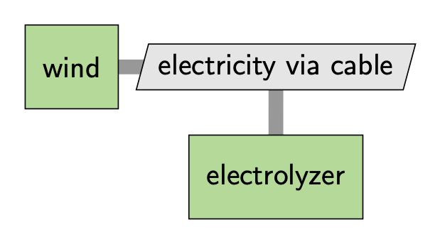
Figure: XDSM diagram generated from the technology interconnections.
N2 diagram (interactive and complete)#
Use OpenMDAO’s n2 utility to generate an interactive HTML diagram of the full model.
from h2integrate.core.h2integrate_model import H2IntegrateModel
import openmdao.api as om
import os


# Change to an example directory
os.chdir("../../examples/08_wind_electrolyzer/")

# Build and set up the model
h2i_model = H2IntegrateModel("wind_plant_electrolyzer.yaml")
h2i_model.setup()

# Write interactive N2 HTML diagram
om.n2(
    h2i_model.prob,
    outfile="h2i_n2.html",
    display_in_notebook=False, # set to True to display in-line in a notebook
    show_browser=False, # set to True to open in a browser at run time
)
Open h2i_n2.html in a browser to explore model groups, components, and variable connections.
Figure: Interactive OpenMDAO N2 diagram showing the full model structure and variable connections.
Running the analysis#
Once you have the config files defined, you can run the analysis using a simple Python script that inputs the top-level config yaml. Here, we will show a script that runs one of the example analyses included in the H2Integrate package.
from h2integrate.core.h2integrate_model import H2IntegrateModel
import os


# Change the current working directory
os.chdir("../../examples/08_wind_electrolyzer/")

# Create a H2Integrate model
h2i_model = H2IntegrateModel("wind_plant_electrolyzer.yaml")

# Run the model
h2i_model.run()

# h2i_model.post_process()

# Print the average annual hydrogen produced by the electrolyzer in kg/year
annual_hydrogen = h2i_model.model.get_val("electrolyzer.annual_hydrogen_produced", units="kg/year").mean()
print(f"Total hydrogen produced by the electrolyzer: {annual_hydrogen:.2f} kg/year")
Total hydrogen produced by the electrolyzer: 51724447.55 kg/year
This will run the analysis defined in the config files and generate the output files in the through the post_process method.
Modifying and rerunning the analysis#
Once the configs are loaded into H2I and the model is instantiated, you can directly modify the underlying OpenMDAO variables within H2I. This is an advanced approach that isn’t necessarily recommended for basic users, but showcases the level of flexibility possible with H2I.
Note
The same behavior shown here with a manual for-loop can be achieved by using the design of experiments capability.
# Access the configuration dictionaries
tech_config = h2i_model.technology_config

# Modify a parameter in the technology config
tech_config["technologies"]["electrolyzer"]["model_inputs"]["performance_parameters"][
    "n_clusters"
] = 15

# Rerun the model with the updated configurations
h2i_model.run()

# Post-process the results
# h2i_model.post_process()

# Print the average annual hydrogen produced by the electrolyzer in kg/year
annual_hydrogen = h2i_model.model.get_val("electrolyzer.annual_hydrogen_produced", units="kg/year").mean()
print(f"Total hydrogen produced by the electrolyzer: {annual_hydrogen:.2f} kg/year")
Total hydrogen produced by the electrolyzer: 51724447.55 kg/year
This is especially useful when you want to run an H2I model as a script and modify parameters dynamically without changing the original YAML configuration file. If you want to do a simple parameter sweep, you can wrap this in a loop and modify the parameters as needed.
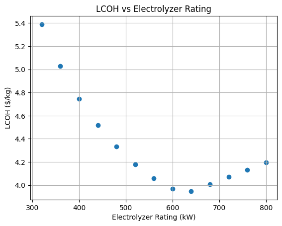
In the example below, we modify the electrolyzer n_clusters and plot the impact on the LCOH.
import numpy as np
import matplotlib.pyplot as plt

# Get the electrolyzer cluster rated capacity
cluster_size_mw = int(
    tech_config["technologies"]["electrolyzer"]["model_inputs"]["performance_parameters"][
        "cluster_rating_MW"
    ]
)

# Define the range for electrolyzer rating
ratings = np.arange(320, 840, cluster_size_mw)

# Initialize arrays to store results
lcoh_results = []

for rating in ratings:
    # Calculate the number of clusters from the rating
    n_clusters = int(rating / cluster_size_mw)

    # Set the n_clusters value directly
    h2i_model.model.set_val("electrolyzer.n_clusters", n_clusters)

    # Rerun the model with the updated configurations
    h2i_model.run()

    # Get the LCOH value
    lcoh = h2i_model.model.get_val("finance_subgroup_hydrogen.LCOH_produced_custom_model", units="USD/kg")[0]

    # Store the results
    lcoh_results.append(lcoh)

# Create a scatter plot
plt.scatter(ratings, lcoh_results)
plt.xlabel("Electrolyzer Rating (kW)")
plt.ylabel("LCOH ($/kg)")
plt.title("LCOH vs Electrolyzer Rating")
plt.grid(True)
plt.show()